Boundary Value Problem

강좌: 수치해석

Boundary Value Problem

IVP와 달리 미분 방정식의 양끝단에서 값이 주어진 문제가 있다.

\[ \frac{dy}{dt}=f(x, y(x)), x \in (a,b), g(y(a), y(b)) = 0. \]

IVP와 같이 미분방정식을 적분해야 하나, 양끝단에 조건이 만족할 수 있어야 한다.

크게 2가지 방법으로 ‘Shooting method’ 와 ‘Finite Difference method’ 가 사용된다.

예제

다음 예제에 대해서 이들 방법을 설명하고자 한다.

금속 막대에 열전달이 발생하는 경우 Fick’s Law에 의해 다음 방정식이 만족한다.

\[ \frac{dT^2}{dx^2} + h(T_a - T) = 0. \]

이때 경계조건은

\[ T(0) = T_1, T(L) = T_2. \]

10m 막대에 대해 다음 변수들로 생각하자. \(T_a=20, T_1= 40, T_2=200, h=0.01\).

이때 이론해는 다음과 같다.

\[ T=73.4523e^{0.1x} - 53.4523e^{-0.1x} + 20. \]

%matplotlib inline
from matplotlib import pyplot as plt
from scipy.integrate import solve_ivp

import numpy as np

plt.style.use('ggplot')
plt.rcParams['figure.dpi'] = 150

# Exact solution
def exact(x):
    return 73.4523*np.exp(0.1*x) - 53.4523*np.exp(-0.1*x) + 20

x = np.linspace(0, 10, 101)

# Plot Exact solution
plt.plot(x, exact(x))
plt.legend('Exact')
plt.xlabel('x')
plt.ylabel('y')

Text(0, 0.5, 'y')

Shooting method

Shooting method는 IVP를 푸는데, 안주어진 초기 조건을 가정해서 경계조건을 만족하도록 shooting 하는 방법이다.

위 예제를 IVP로 풀 경우 다음과 같이 고차 미분항을 보조변수를 이용해 표현한다.

\[\begin{split} \begin{align} \frac{dT}{dx} &= z \\ \frac{dz}{dz} &= h(T-T_a) \end{align} \end{split}\]

초기조건으로 \(T(0)=T_1\) 주어졌으나 \(z(0)\)는 주어지지 않아서 이를 가정해서 푼다.

solve_ivp를 이용해서 이를 구현하면 다음과 같다.

# Constants
Ta, T1, T2 = 20, 40, 200
h = 0.01

# derivative function
def dydx(t, y):
    # y[0], y[1] : T and z
    return np.array([y[1], h*(y[0] - Ta)])

# z(0)가 0일 때 해석
z1 = 0
sol1 = solve_ivp(dydx, t_span=(0, 10), y0=[T1, z1], t_eval=x)

# Print result
print(sol1)

# T2
print("T(L) for guess z0={:.3f}: {:.3f}".format(z1, sol1.y[0][-1]))

  message: The solver successfully reached the end of the integration interval.
  success: True
   status: 0
        t: [ 0.000e+00  1.000e-01 ...  9.900e+00  1.000e+01]
        y: [[ 4.000e+01  4.000e+01 ...  5.063e+01  5.086e+01]
            [ 0.000e+00  2.000e-02 ...  2.320e+00  2.350e+00]]
      sol: None
 t_events: None
 y_events: None
     nfev: 32
     njev: 0
      nlu: 0
T(L) for guess z0=0.000: 50.862

# z(0)가 0일 때 해석
z1 = 20
sol2 = solve_ivp(dydx, t_span=(0, 10), y0=[T1, z1], t_eval=x)

# T2
print("T(L) for guess z0={:.3f}: {:.3f}".format(z1, sol2.y[0][-1]))

T(L) for guess z0=20.000: 285.897

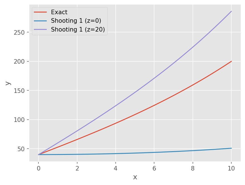
초기 추측값으로 실험한 결과 \(z_0 \in (0, 20)\) 일 때 해가 존재한다.

\(z_0\) 값을 바꿔도 되지만, 이를 root finding 기법으로 찾아보자.

root_scalar 함수를 활용하자.

# Plot results of initial guess
plt.plot(x, exact(x))
plt.plot(sol1.t, sol1.y[0])
plt.plot(sol2.t, sol2.y[0])

plt.legend(['Exact', 'Shooting 1 (z=0)', 'Shooting 1 (z=20)'])
plt.xlabel('x')
plt.ylabel('y')

Text(0, 0.5, 'y')

from scipy.optimize import root_scalar


# Root finding function
def obj(z):
    sol = solve_ivp(dydx, t_span=(0, 10), y0=[T1, z])
    return sol.y[0][-1] - T2


# root finding (Bracketing method)
root = root_scalar(obj, bracket=[0, 20])
print(root)

      converged: True
           flag: 'converged'
 function_calls: 6
     iterations: 5
           root: 12.690853836888637

# Solve IVP with the root z
sol = solve_ivp(dydx, t_span=(0, 10), y0=[T1, root.root])

# Plot the result of shooting method
plt.plot(x, exact(x))
plt.plot(sol.t, sol.y[0], marker='x', linestyle='none')

# Legend and labels
plt.legend(['Exact', 'Shooting 1 (z={:.3f})'.format(root.root)])
plt.xlabel('x')
plt.ylabel('y')

Text(0, 0.5, 'y')

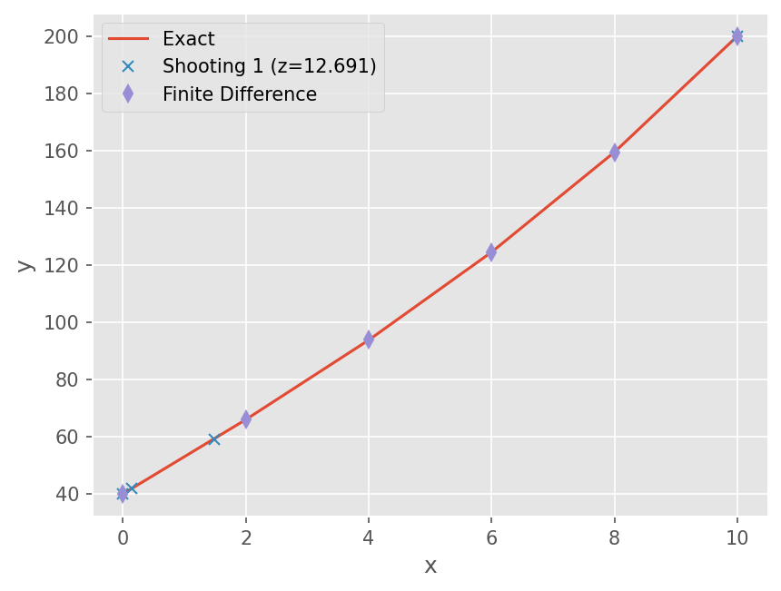
Finite Differenece Method

Finite Difference 를 적용하면 양 끝점 사이 \(x\) 를 n 등분 한다.. 이 때 미분을 Finite difference로 표현하면 다음과 같다.

\[ \frac{T_{i+1} - 2 T_i + T_{i-1}}{\Delta x^2} - h(T_i - T_a) = 0. \]

이를 정리하면 다음과 같다

\[ -T_{i-1} + (2 + h \Delta x^2) T_i - T_{i+1} = h \Delta x^2 T_a \]

양 끝점의 값은 \(T_0\), \(T_{n}\) 이다.

각 점에서 이 식을 전개하면 다음과 같다.

\[\begin{split} \begin{align} &+ (2 + h \Delta x^2) T_1 &- T_{2} &= h \Delta x^2 T_a + T_0 \\ -T_{1} &+ (2 + h \Delta x^2) T_2 &- T_{3} &= h \Delta x^2 T_a \\ & & ... & & \\ -T_{n-3} &+ (2 + h \Delta x^2) T_{n-2} &- T_{n-1} &= h \Delta x^2 T_a \\ -T_{n-2} &+ (2 + h \Delta x^2) T_{n-1} & &= h \Delta x^2 T_a + T_{n} \end{align} \end{split}\]

n-1 개의 연립방정식을 해석한다. 위 예제를 적용하면 다음과 같다.

\[\begin{split} \left [ \begin{array}{cccc} (2 + h \Delta x^2) & -1 & 0 & 0 & ... & 0 \\ -1 & (2 + h \Delta x^2) & -1 & 0 & ... \\ 0 & & ... & & \\ 0 & & ... & -1 &(2 + h \Delta x^2) & -1 \\ 0 & & ... & & -1 & (2 + h \Delta x^2) \end{array} \right ] \left [ \begin{array}{c} T_1 \\ T_2 \\ ...\\ T_{n-2} \\ T_{n-1} \end{array} \right ] = \left [ \begin{array}{c} h \Delta x^2 T_a + T_0 \\ h \Delta x^2 T_a \\ ... \\h \Delta x^2 T_a \\h \Delta x^2 T_a + T_n \end{array} \right ] \end{split}\]

linalg.solve 함수를 활용해서 해석하는 코드는 다음과 같다.

# Number of division
n = 5

# Array x
x = np.linspace(0, 10, n+1)
dx = np.diff(x)[0]

# Array y
y = np.empty_like(x)
y[0], y[-1] = T1, T2

# Operator
A = np.zeros((n-1, n-1))

for i in range(n-1):
    A[i, i] = 2 + h*dx**2
    if i > 0:
        A[i, i-1] = -1
    if i < n-2:
        A[i, i+1] = -1

# Forcing term
b = np.ones(n-1)
b *= h*dx**2*Ta
b[0] += T1
b[-1] += T2

# Solve system
y[1:-1] = np.linalg.solve(A, b)
print(y)

[ 40.          65.96983437  93.77846211 124.53822833 159.47952369
 200.        ]

# Plot numerical results
plt.plot(x, exact(x))
plt.plot(sol.t, sol.y[0], marker='x', linestyle='none')
plt.plot(x, y, marker='d', linestyle='none')

# Legend and Labels
plt.legend(['Exact', 'Shooting 1 (z={:.3f})'.format(root.root), 'Finite Difference'])
plt.xlabel('x')
plt.ylabel('y')

Text(0, 0.5, 'y')

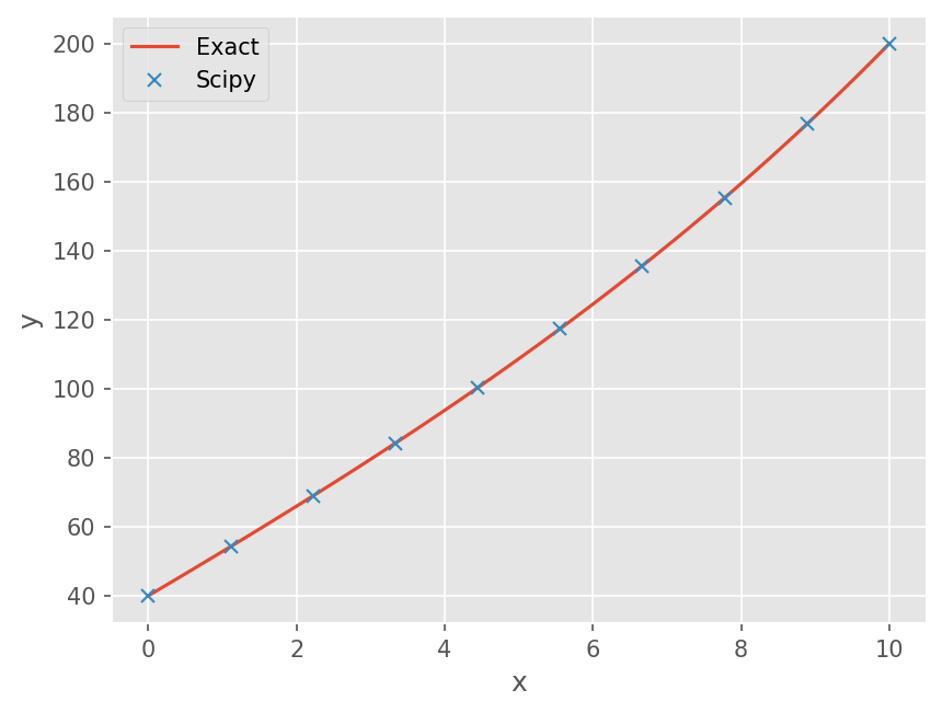
Scipy 활용

scipy.integrate 모듈 내 BVP 해석 함수도 제공한다.

boundary value problem

solve_bvp 함수는 경계 조건에 맞게 미분 방정식을 수치적으로 해석한다

from scipy.integrate import solve_bvp

# derivative function
def dydx(t, y):
    # y[0], y[1] : T and z
    return np.array([y[1], h*(y[0] - Ta)])

# Boundary condition
def bc(ya, yb):
    # both ends point as ya and yb
    return np.array([ya[0] - T1, yb[0] - T2])

# Array x
n = 10
x = np.linspace(0, 10, n)
y = np.zeros((2, n))

sol = solve_bvp(dydx, bc, x ,y)

# Plot numerical results
x = np.linspace(0, 10, 101)
plt.plot(x, exact(x))
plt.plot(sol.x, sol.y[0], marker='x', linestyle='none')

# Legend and Labels
plt.legend(['Exact', 'Scipy'])
plt.xlabel('x')
plt.ylabel('y')

Text(0, 0.5, 'y')